Linear Regression
Definition
Suppose $y$ is terget value vector, $X$ is input matrix. X has n samples and each sample has m features with 1 intercept.
\[y = \left[\begin{matrix} y_1\\ y_2\\ ...\\ y_n \end{matrix} \right]\] \[X = \left[\begin{matrix} 1 & x_{11} & x_{12} &... & x_{1m}\\ 1 & x_{21} & x_{22} &... & x_{2m}\\ : & : & : & : & :\\ 1 & x_{n1} & x_{n2} &... & x_{nm} \end{matrix} \right]\]The first column of X is for intercept. The basic linear regression is to find a coefficients vector $w$ so that
\[\left[\begin{matrix} 1 & x_{11} & x_{12} &... & x_{1m}\\ 1 & x_{21} & x_{22} &... & x_{2m}\\ : & : & : & : & :\\ 1 & x_{n1} & x_{n2} &... & x_{nm} \end{matrix} \right] * \left[\begin{matrix} w_0\\ w_1\\ ...\\ w_m \end{matrix} \right] =\left[\begin{matrix} y_1\\ y_2\\ ...\\ y_n \end{matrix} \right]\]In short hand, $X*w = y$. In most cases, there is no such $w$ satisfy the equation. Since $X$ is not square matrix then it’s not invetible. We cannot simply calculate $w = X^{-1}y$.
Ordinary Least Squares
Since there is no exactly matched $w$, so we can only try our best to find optimal $w$. Intuitively, the optimal $w$ should minimize the distance between the dots and line.
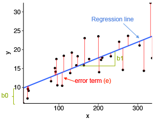
The length of red line is:
\[|y_i - x_iw|\]Then we can define our loss function as:
\[J(w) = \sum_{i = 1}^n(y_i - x_iw)^2 = (y-Xw)^T(y-Xw)\]Take derivative on $w$:
\[\frac{\partial J}{\partial w} = -2X^T(y-Xw) = 0\]As a result:
\[X^T(y-Xw)= 0\\X^Ty - X^TXw = 0\\ X^TXw = X^Ty\\ w = (X^TX)^{-1}X^Ty\]Digging into OLS - Probability
Why we use sum of square but not absolute value or third/ fourth power?
Everything comes from maximum likelihood estimation!
There is implied assumption - the residuals are normally distributed!
Denote $y_i$ is true value, $\hat{y}_i$ is estimated value.
\[\epsilon_i = y_i - \hat{y}_i\\ \epsilon \sim N(0,\sigma^2)\]Which means: \(y_i \sim N(x_iw,\sigma^2)\)
So the probability for $y_i$ is:
\[p(y_i) = \frac{1}{\sqrt{2\pi}\sigma}*exp[-\frac{(y_i - x_iw)^2}{2\sigma^2}]\]Then the likelihood function is:
\[L(w) = \prod_{i=1}^n \frac{1}{\sqrt{2\pi}\sigma}*exp[-\frac{(y_i - x_iw)^2}{2\sigma^2}]\]The log likelihood function would be:
\[L(w) = - n\log\sigma - \frac{n}{2}log2\pi - \sum_{i=1}^n\frac{(y_i - x_iw)^2}{2\sigma^2}\]Since the first two items are fixed, so maximize the L(w) is equal to minimize $(y_i - x_iw)^2$. And it’s same as OLS. In other words, OLS estimator also maximize likelihood function.
Digging into OLS - Econometrics
In statistic, a good estimation should be BLUE (unbiased and smallest variance).
Below are assumptions MLR 1- 6
- Linear in Parameters
- Random Sampling
- No perfect Colinearity
- Zero Conditional Mean
- Homoskedasticity
- Normality of Error Term
Express MLR 4-6 in mathmatic language:
\[E(u|x_1,x_2..x_n) = 0\] \[Var(\epsilon|x_1,x_2...x_n) = \sigma^2\] \[\epsilon \sim N(0,\sigma^2)\]Under MLR 1-4, the estimators are unbiased.
\[E(\hat w_i) = w_i\]Under MLR 1-5, the estimators are effectiveness.
Also, under MLR 1-5, we can estimate the variance of coefficients ($Var(\hat w_i)$) and error term($\hat\sigma^2$).
Under MRL 1-6, the estimators are normally distributed. Then we can do hypothesis test, p value or cofidence interval.
\[\hat w_i \sim N(w_i,Var(\hat w_i))\]Because of center limit theory, we can lose our assumption when the sample size is large. Large sample + MLR 1-5 can also get above properties.
References
标准与局部加权线性回归
岭回归和LASSO
脊回归(Ridge Regression)
线性回归(Linear Regression)
Lasso回归和岭(Ridge)回归
简单易学的机器学习算法——岭回归(Ridge Regression)
线性回归损失函数为什么要用平方形式