Time Series Analysis Basics
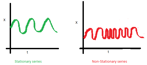
Stationary Series
Three creterias for stationary series:
- The mean of series should be constant but not a function of time.
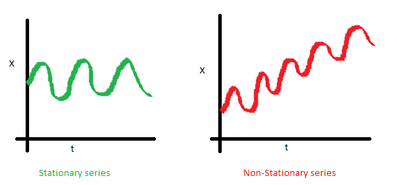
- The variance of series should not be a function of time, in economics, it’s called homescedasticity.
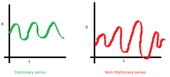
- The covariance of i th term and the (i + m) th term should not be a function of time.
Why stationary series so important?
It cannot be modeled unless it’s stationary series. Typically, the first step is stationarizing the time series. The methods include Detrending, Differencing etc.
Random Walk
Suppose $X$ represent a stochastic number (also can be viewed as time series data) and has following feature:
\[dX = dW\]Which means the movement of $X$ is purely random and $X$ is random walk.
Assume at time 0, the value of $X$ is known as $X_0$. We can write down the expression of $X_t$.
\[X_t = X_0 + \int_0^tdW_t\]As a result, $X_t$ has following chracteristics:
- Mean Constant
\(E(X_t) = X_0\)
- Time Varing Variance
So $X$ is not a stationary process
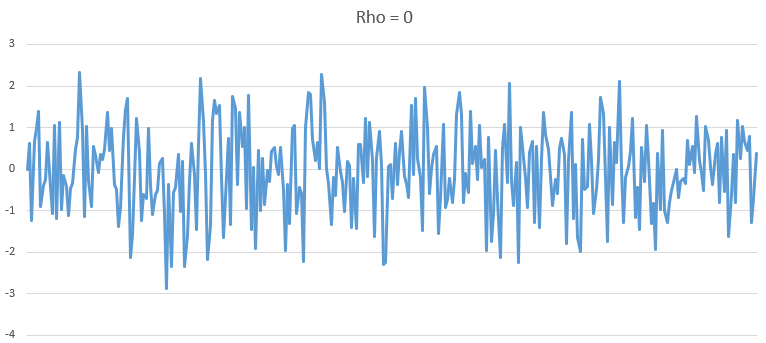
Rho Coefficient and ADF Test
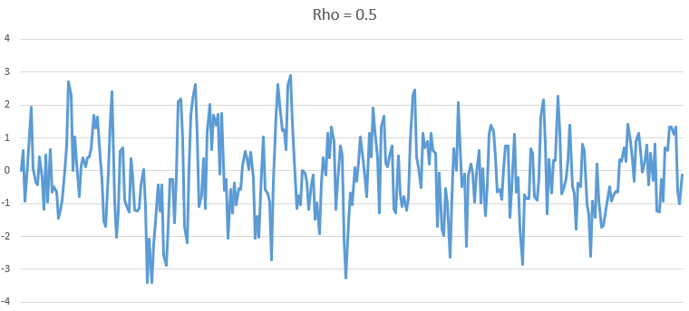
\[X_t = Rho*X_{t-1} + W_{t-(t-1)}\]If Rho = 0,here is the plot for the time series:
Rho = 0.5
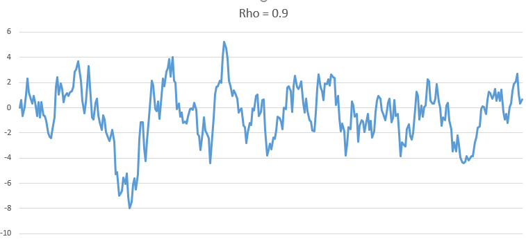
Rho = 0.9
Rho = 1
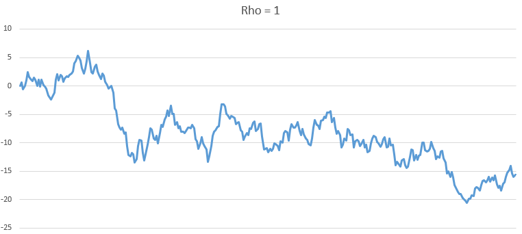
As we can see, as Rho increase, the series becomes more and more non-stationary.
Take the expectation:
\[E(X_t) = Rho * E(X_{t-1})\]If Rho is less than 1, then X is pulled back to 0. For example, $X_{t-1} = 2$ and $Rho = 0.5$, then $E(X_t) = 1$.
Rearrange the equation we get:
\[X_t - X_{t-1} = (Rho-1)*X_{t-1} + W_{t-(t-1)}\]Then we can do Dickey Fuller Test of Stationarity. Run the regression and do hypothesis test.
Null hypothesis: (Rho-1) equals zero. Alternative hypythesis: (Rho-1) is significantly different than zero.
If reject null hypothesis, which means rho is not 1, the series is stationary.
Stric Stationary and Weak Stationary
Suppose $X_t$ is a time series. For any n, m and k, if the joint distribution of $Z_n, Z_{n-1} … Z_ {m}$ is the same as $Z_{n-k}, Z_{n-k-1} … Z_ {m-k}$. ($n>m$) Then it’s defined as stric stationary.
For weak stationary, it has to satisfy two requirements:
- The mean of time series is constant over time..
- Covariance stationary. The autocovariance is the same for all times and lags k. Simpliy speaking, if lags k is decided, the autocov should be the same.
Make time series stationary
There are 2 major reasons behind non-stationary time series:
- Trend - varying mean over time.
- Seasonality - variations at specific time-frames.
Tricks 1 - Transformation
Take a log on time series data which penalize higher values more than smaller values.
Tricks 2 - Elimilate Trend
The first step is modeling the trend, there are several technics:
- Aggregation - taking average for a time period
- Smoothing - taking rolling averages
- Polynomial Fitting - fit a regression model
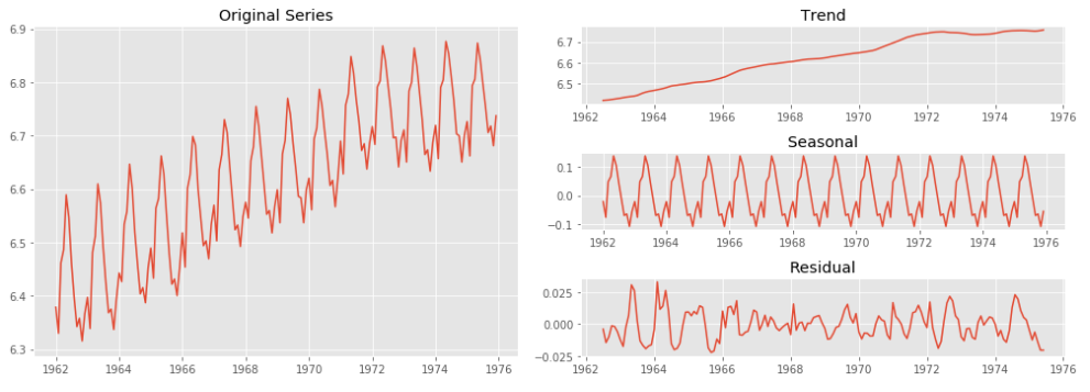
Tricks 3 - Handling Trend and Seasonality
There are mainly two approach:
- Differencing
- Decomposition
Time Series Modeling
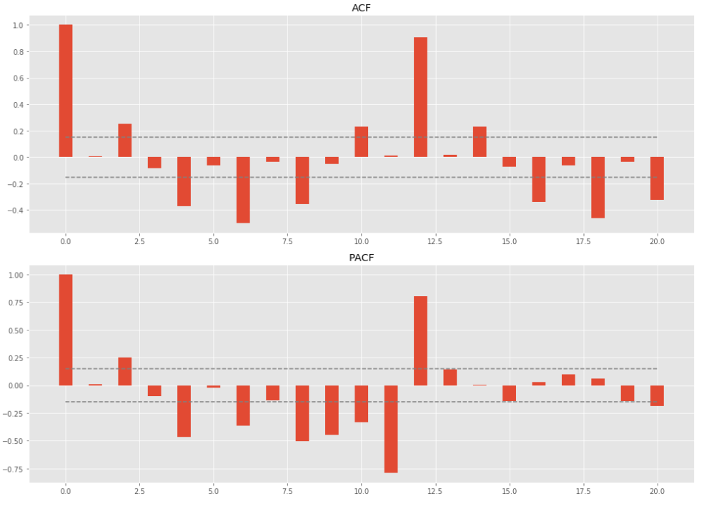
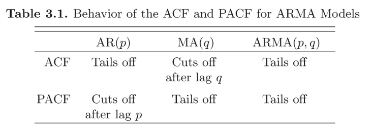
ARIMA Model Parameters Determining
- ACF measures the correlation between the time series and a lagged version of itself.
- PACF measures the correlation between the TS with a lagged version of itself but after eliminating the variations already explained by the intervening comparisons. For example, ACF between $X_t$ and $X_{t-k}$ is not their pure correlation, since $X_t$ are also affected by $X_{t-1}, X_{t-2}…X_{t-k+1}$. PACF is the correlation which elimilate these affections.tions.
Creteria
Quantitative Model Selection - Information Creteria
As we increase the parameters in the model, the performance tends to be better, but we need to penalize the new parameters. There are two common infomation creteria AIC (Akaike Information Criterion) and BIC (Bayesian Information Criterion).
Suppose k is the number of parameters, n is the sample size and L is likelihood function. For AIC:
\[AIC = 2k - 2Ln(L)\]For BIC:
\[BIC = kLn(n) - 2Ln(L)\]The less AIC/BIC the better the model.
Codes
Codes and PDF version of this article can be found from my github repo: BlogPDF
References
A Complete Tutorial on Time Series Modeling in R
A comprehensive beginner’s guide to create a Time Series Forecast (with Codes in Python)