1. Introduction of Black Litterman Framework
The Black-Litterman asset allocation model, created by Fischer Black and Robert Litterman, is a sophisticated portfolio construction method that overcomes the problem of tranditional Mean-Variance Asset Allocation.
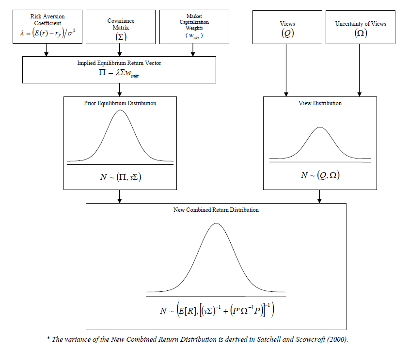
The Black-Litterman model uses a Bayesian approach to combine the subjective views of an investor regarding the expected returns of one or more assets with the market equilibrium vector of expected returns (the prior distribution) to form a new, mixed estimate of expected returns.
Below is the picture summerizes the whole framework:
1.1 Drawbacks of Mean-Variance Asset Allocation
- Highly-concentrated portfolios Large long or short positions
- Input-sensitivity Small change in expected returns will result in large weight change
- Estimation error maximization
These three related and well-documented problems are most likely the reasons that why practitioners do not use it in industry.
1.2 Article Structure
The remaining article will introduce the Black Litterman by following logic:
- Neutral Start Point - Implied Equilibrium Return
- How to quantify investors’ view
- How to combine investors’ view and neutral strat point
2. Neutral Starting Point for Black Litterman Framework
2.1 Implied Equilibrium Return
Suppose the investors have the following utility function:
\[U = w^T\mu - \frac{1}{2} \lambda w^T\Sigma w\]Where w - The weights of the assets $\mu$ - A vector of excess returns $\Sigma$ - Varaince-Covariance matrix of excess returns
To maximize the utility function, we can take the first derivative on U:
\[\frac{\partial U}{\partial w} = \mu - \lambda \Sigma w = 0\]As a result
\[\mu = \lambda \Sigma w\]If we replace the $w$ with market capitalization weight $w_{mkt}$, the corresponding excess return vector is Implied Equilibrium Return Vector. Denote it as $\Pi$.
\[\Pi = \lambda \Sigma w_{mkt}\]If we take this Implied Equilibrium Return Vector as input for optimization, we will get market captalization weights. This is so-called reverse optimization.
For Black Litterman framework, this “Equilibrium” returns is a neutral starting point. By this way, the Black Litterman Model solves the input-sensitivity problem.
2.2 Uncertainty about Equilibrium Returns
The variance of Implied Equilibrium Return is calculated as $\tau \Sigma$. $\tau$ is a scalar, if it’s large, it means that investors are more uncertain about the equilibrium returns.
There are several ways to set up the $\tau$.
2.2.1 Black and Litterman (1992) and Lee (2000)
In the original paper, the Black and Litterman argue that One would expect the Equilibrium Returns to be less volatile than the historical returns. So the $\tau$ should close to 0.
Lee who has considerable experience working with a variant of the Black-Litterman model, typically sets the value of the scalar (τ ) between 0.01 and 0.05, and then calibrates the model based on a target level of tracking error
2.2.2 Satchell and Scowcroft (2000)
Satchell and Scowcroft say the value of the scalar ($\tau$) is often set to 1.
2.2.3 Blamont and Firoozye (2003)
Blamont and Firoozye interpret τΣ as the standard error of estimate of the Implied Equilibrium Return Vector ( Π ); thus, the scalar (τ ) is approximately 1 divided by the number of observations.
2.2.4 He and Litterman (1999)
He and Litterman (1999) calibrate the confidence of a view so that the ratio of $\frac{\omega}{\tau}$ is equal to the variance of the view portfolio ($P_i\Sigma P_i$).
By this way, the $\omega_i$ is calculated as follows:
\[\omega_i = \tau P_i\Sigma P_i\]So no matter what the $\tau$ value is, the final result is the same. The final result only depends on the ratio of $\frac{\omega}{\tau}$.
3. Quantify Investors’ View
There are two kind of investors’ view: absolute and relative. Suppose there are 4 assets: A, B, C and D. $R_x$ represents the return for asset x.
3.1 Relative View
For example, asset A will outperform asset B by 25 base points is a relative view. In mathmatic language, it can be written as:
\[R_a - R_b = 0.0025\]In linear algebra, it’s:
\[\begin{bmatrix} 1 & -1 & 0 & 0 \end{bmatrix} \begin{bmatrix} R_a \\ R_b \\ R_c \\ R_d \end{bmatrix} = 0.0025\] \[P_i * R = Q_i\]Where
$P_i$ is the row vector for ith view.
$Q_i$ is the value of the ith view.
Intuitively, each view can be taken as a mini long/short portfolio with weights sum to 0.
3.2 Absolute View
For example, asset C will have an absolute excess return of 5.25% is a absolute view.
Also, it can be expressed in linear algebra:
\[\begin{bmatrix} 0 & 0 & 1 & 0 \end{bmatrix} \begin{bmatrix} R_a \\ R_b \\ R_c \\ R_d \end{bmatrix} = 0.0525\]And we still use $P_i$ and $Q_i$ for deonotation.
Note: Since the absolute view portfolio doesn’t sum to 0, the final portfolio weights will not sum to 1.
3.3 Denotation for several views
Investor can have several views at the same time, suppose there are n views. It be can denote as follow:
\[P = \begin{bmatrix} P_1 \\ P_2 \\ \vdots \\ P_n \end{bmatrix}\ \ \ \ \ \ \ Q = \begin{bmatrix} Q_1 \\ Q_2 \\ \vdots \\ Q_n \end{bmatrix}\]3.4 Uncertainty about views
In Black Litterman Model, it assumes that the error term of views follow gaussian distribution. And views are indepent.
The Black Litterman Model calcualte the variance of individual view in the following way:
\[\omega_i = P_i\Sigma P_i\]The covariance matrix of all the error terms has the following form:
\[\Omega = \begin{bmatrix} \omega_1 &0&0&\cdots&0\\ 0&\omega_1 &0&\cdots&0 \\ \vdots&\vdots&\vdots&\ddots&\vdots \\ 0&0&0&\cdots&\omega_n \end{bmatrix}\]The zeros in the off-diagnol are because the views are independent.
4. Combined Returns
So far, we have the following inputs:
- $\Pi$ - Implied Equilibrium Return Vector
- $\tau \Sigma$ - Variance of Equilibrium Return
- $P$ - a matrix that identifies the assets involved in the views
- $Q$ - the View Vector
- $\Omega$ - Diagonal Covariance Matrix which specify the Variance of Views
The formula for the combined returns $E[R]$ is:
\[E[R] = [(\tau \Sigma)^{-1}+P^T \Omega^{-1}P]^{-1}[(\tau \Sigma)^{-1}\Pi + P^T \Omega^{-1}Q]\]Interpretation
$[(\tau \Sigma)^{-1}\Pi + P^T \Omega^{-1}Q]$ can be viewed as the weighted average of $\Pi$ and $Q$
$(\tau \Sigma)^{-1}$ is the weight for $\Pi$
$P^T \Omega^{-1}$ is the weight for $Q$
If investors are more certain about views, the relative weight for $Q$ would be higher
$[(\tau \Sigma)^{-1}+P^T \Omega^{-1}P]^{-1}$ is just a scaler to make the weights sum to 1
4.1 Backout the optimized weights
The weights can be back out using the following formula: \(w = (\lambda \Sigma)^{-1}E(R)\)
One of the strongest features of the Black-Litterman model is only the weights of the assets which views were expressed changed from their original market capitalization weights.
He and Litterman (1999) and Litterman (2003) suggest that, in the presence of constraints, the investor input the New Combined Return Vector ( E[R]) into a mean-variance optimizer.
References
A Step-by-Step Guide to The Black-Litterman Model-Thomas M. Idzorek
Best, M.J., and Grauer, R.R. (1991). “On the Sensitivity of Mean-Variance-Efficient Portfolios to Changes in Asset Means: Some Analytical and Computational Results.” The Review of Financial Studies, January, 315-342.
Bevan, A., and Winkelmann, K. (1998). “Using the Black-Litterman Global Asset Allocation Model: Three Years of Practical Experience.” Fixed Income Research, Goldman, Sachs & Company, December.
Black, F. (1989a). “Equilibrium Exchange Rate Hedging.” NBER Working Paper Series: Working Paper No. 2947, April.
Black, F. (1989b). “Universal Hedging: Optimizing Currency Risk and Reward in International Equity Portfolios.” Financial Analysts Journal, July/August,16-22.
Black, F. and Litterman, R. (1990). “Asset Allocation: Combining Investors Views with Market Equilibrium.” Fixed Income Research, Goldman, Sachs & Company, September.
Black, F. and Litterman, R. (1991). “Global Asset Allocation with Equities, Bonds, and Currencies.” Fixed Income Research, Goldman, Sachs & Company, October.
Black, F. and Litterman, R. (1992). “Global Portfolio Optimization.” Financial Analysts Journal, September/October, 28-43.
Blamont, D. and Firoozy, N. (2003). “Asset Allocation Model.” Global Markets Research: Fixed Income Research, Deutsche Bank, July.
Fusai, G. and Meucci, A. (2003). “Assessing Views.” Risk, March 2003, s18-s21. Grinold, R.C. (1996). “Domestic Grapes from Imported Wine.” Journal of Portfolio Management, Special Issue, 29-40.
Grinold, R.C., and Kahn, R.N. (1999). Active Portfolio Management. 2nd ed. New York: McGraw-Hill.
Grinold, R.C. and Meese, R. (2000). “The Bias Against International Investing: Strategic Asset Allocation and Currency Hedging.” Investment Insights, Barclays Global Investors, August